Installing on Windows
On Windows, the easiest way to install HyperSpy is to use the HyperSpy bundle installer. This simple to install program provides a customized Anaconda installation, which contains the HyperSpy libraries but also other libraries used in the field of electron microsocpy. A detailed walk through of the process is provided below.
Download
First, download the installer using the following link (https://github.com/ericpre/hyperspy-bundle/releases):
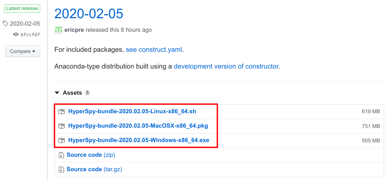
Download the installer corresponding to your system.
Installing
Run the downloaded file to proceed with the installation. This process is fairly straightforward. For the installation location, we highly recommend to install as single user in a folder that does not require administrative rights, as set by default.
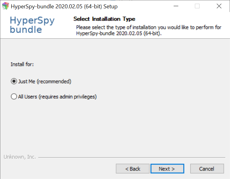
Single user installation is recommended.
It is recommended to install the HyperSpy bundle in a folder with a short path (less than 32 characters) to avoid issues with the JupyterLab and its deeply nested folder structure. The default folder should be fine in most situations (non domain user account):
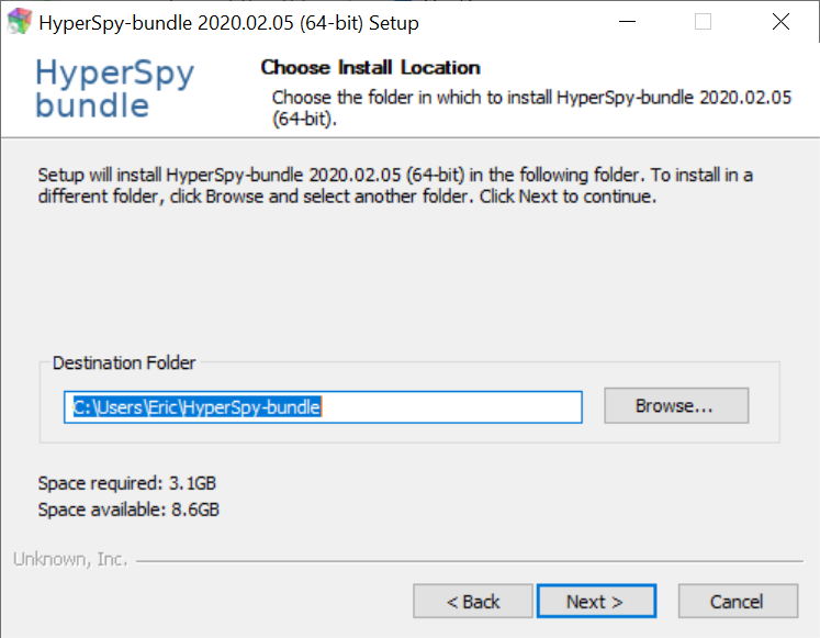
It is recommended to install the HyperSpy bundle in a folder with a short path (less than 32 characters).
Keep the default options unless you know what you are doing:
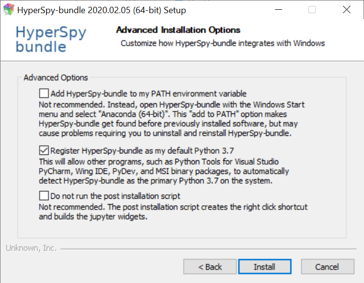
A screenshot showing the default options. If a dfferent Python distribution is installed on the system, by default this distribution will not be registered as the default Python distribution.
Doing so will install HyperSpy into your user folder under a subfolder named
"Anaconda (64 bits)". The installation may take some time, but you should get
a progress window that looks like:
And that’s it! All the installed programs should now be available within the Start Menu under the “HyperSpy Bundle” folder. You can either continue following the next section to test the installation, or continue to the Obtaining the tutorial data section on the main page.
Testing the installation
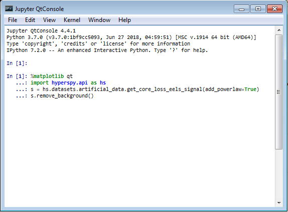
Start the jupyter qconsole using the context menu (right click) short cut, see the Starting HyperSpy section
The Qt Console is an interactive Python interpreter that allows you to enter
Python statements directly and immediately see their output. Once the console
has opened and you see a prompt that says In [1]:, copy the following code
snippet at the location of the blinking cursor:
%matplotlib qt
import hyperspy.api as hs
s = hs.datasets.artificial_data.get_core_loss_eels_signal(add_powerlaw=True)
s.remove_background()
Very briefly, this code is loading the interactive plotting libraries, loading
HyperSpy, creating an example EELS signal from some artificial data, and then
telling the interpreter you want to interactively remove the Power Law
background. Press Shift-Enter within the console to run the lines of code
you pasted in (it may take a few moments to run if this is the first time
you’ve used HyperSpy on your machine):
Entering the example code into the Qt Console
Eventually, you should see a spectrum window and a small tool window for removing the background open (they may be stacked on top of each other; drag them out of the way, if so). If you click and drag on part of the spectrum display, HyperSpy will fit a Power Law to the signal within that region, and also show you a preview of the background-subtracted signal:
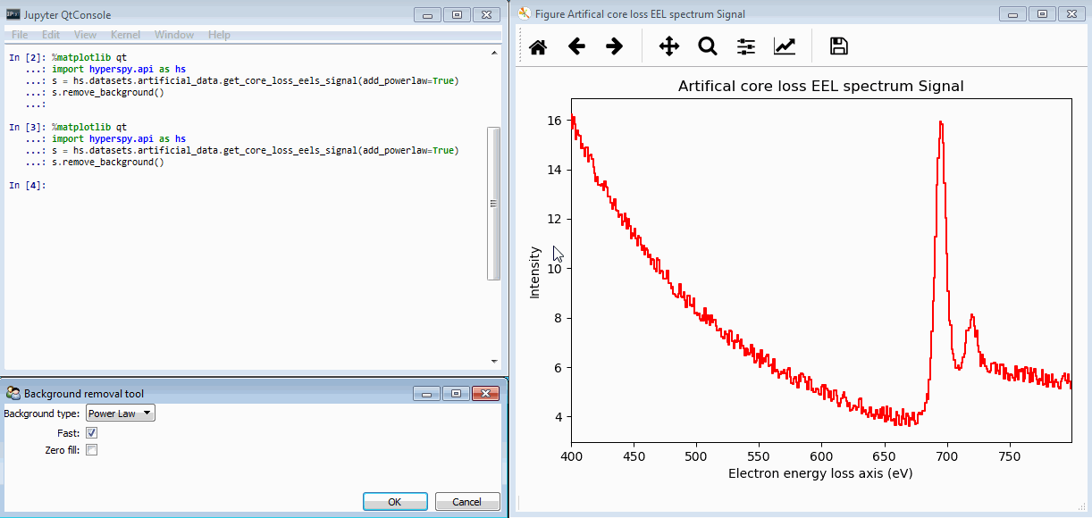
By clicking and dragging on the spectrum display, a region is created (shown in red). The fitted background is shown in blue, and a preview of the background-subtracted signal is displayed in green.
Clicking “OK” in the Background removal tool window will perform the background subtraction, and replace the window with one showing the resulting signal:
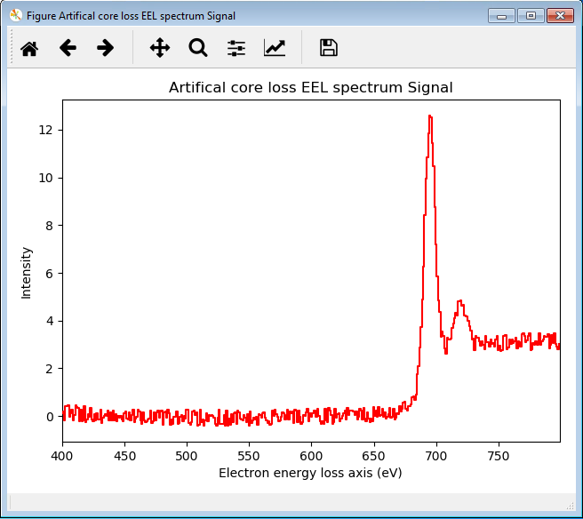
Assuming all of this worked, congratulations! You have a working HyperSpy installation and you have run your first bit of open-source HyperSpy-based materials science data analysis! Click the button below to return to the main tutorial homepage: